
We have explored the dynamics and energy budgets of the oceanic general circulation and its associated mesoscale eddy field in a number of papers employing idealized models, realistic ocean general circulation models, in-situ observations, and satellite observations. Specific topics of interest include the impact of bottom boundary layer drag and topographic wave drag on eddy statistics and eddy dynamics, the oceanic inverse energy cascade, the dynamics of jets and vortices, the use of higher-order stencils to compute geostrophic velocities from altimeter observations of sea surface heights, and comparison of modeled kinetic and potential energies to energies derived from altimeter observations and observations from various in-situ platforms including current meters, drifters, and Argo floats.
Our research focuses on the use of numerical models to better understand the dynamics and energy budgets of both wind- and tidally-forced flows in the ocean.
Back to All ResearchHe Wang
Personnel details dialog.
He Wang
Project Scientist II at UCAR
He joined our group in 2020. He works on tide modeling and Great Lakes modeling using the NOAA MOM6 ocean model.
Research Projects
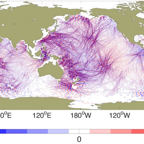
Global modeling of internal tides and the internal gravity wave continuum
Most Recent Group Publications
96 – The Chicxulub impact produced a powerful global tsunami
110 – Improving global barotropic tides with sub-grid scale topography
Badarvada Yadidya
Personnel details dialog.
Badarvada Yadidya
Postdoctoral Fellow
Yadidya joined our group in 2023 after obtaining his PhD at IIT New Delhi. He is exploring the phase accuracy of internal tides in US Navy HYCOM forecasts.
Most Recent Group Publications
129 – Advancing internal tide correction for SWOT Cal/Val: The role of ocean forecasts
Siva Heramb Peddada
Personnel details dialog.
Siva Heramb Peddada
Postdoctoral Fellow
Siva joined our group in 2024. He is exploring the use of ocean models to map ocean mixing.
Hugo Plombat
Personnel details dialog.
Hugo Plombat
Postdoctoral Fellow
Hugo received his PhD from Université de Montpellier in Astrophysics. He joined our group in 2024 and his project connects lunar orbit evolution with ocean tide modeling.
Julia (Jia-Xuan) Chang
Personnel details dialog.
Julia (Jia-Xuan) Chang
Postdoctoral Fellow
Julia recieved her PhD from University of Victoria and joined our group in 2025. She is working on analysis of SWOT data and models.
Joseph Ansong
Personnel details dialog.
Joseph Ansong
Former Postdoctoral Fellow
Joseph received his PhD in Applied Mathematics from the University of Alberta. Joseph was a postdoc and then research scientist in our group from 2011-2017. He is now a Lecturer (equivalent of assistant professor) at the University of Ghana.
Amanda O'Rourke
Personnel details dialog.
Amanda O'Rourke
Former Postdoctoral Fellow
Amanda received her PhD in Atmospheric and Oceanic Sciences from Princeton University. Amanda was in our group from 2014-2017. She is now a scientist at the Johns Hopkins University Applied Physics Laboratory.
Patrick Timko
Personnel details dialog.
Patrick Timko
Former Postdoctoral Fellow
Patrick received his PhD in Physical Oceanography from Memorial University of Newfoundland. Patrick was a postdoc in our group from 2008-2012. He is now a Support Scientist at Environment Canada.
David Trossman
Personnel details dialog.
David Trossman
Former Postdoctoral Fellow
David was in our group from 2011-2013, after receiving his PhD in Physical Oceanography from the University of Washington. David is now a Visiting Associate Research Scientist at NOAA STAR/NESDIS Laboratory for Satellite Altimetry (LSA; through the cooperative agreement between NOAA and University of Maryland-College Park).
Research Projects
Dynamics and energy budgets of oceanic general circulation and mesoscale eddies
Global modeling of internal tides and the internal gravity wave continuum
Most Recent Group Publications
68 – Connecting process models of topographic wave drag to global eddying general circulation models
Arin Nelson
Personnel details dialog.
Arin Nelson
Former Postdoctoral Fellow
Arin received his PhD in Atmospheric and Oceanic Sciences from the University of Colorado. Arin was in our group from 2017-2020. He worked on non-phase-locked internal tides and on high-resolution internal gravity wave modeling. He is now a scientist at the Naval Undersea Warfare Center.
Most Recent Group Publications
Ritabrata Thakur
Personnel details dialog.
Ritabrata Thakur
Former Postdoctoral Fellow
Ritabrata joined our group in 2020. He worked on high-resolution internal wave models and is now on the faculty of IIT New Delhi.
Most Recent Group Publications
Joseph Skitka
Personnel details dialog.
Joseph Skitka
Former Postdoctoral Fellow
Joe joined our group in 2020. He worked on the dynamics and energy budgets of the internal wave spectrum in models.
Most Recent Group Publications
Malte Müller
Personnel details dialog.
Malte Müller
Former Postdoctoral Scientist
Malte received his PhD in Oceanography from the University of Hamburg. He worked with us from 2012-2013 as a postdoctoral contractor. Malte is now a Research Scientist at the Norwegian Meteorological Insitute.
Research Projects
Variability of the coupled atmosphere-ocean system
Global modeling of internal tides and the internal gravity wave continuum
Anthony Chen
Personnel details dialog.
Anthony Chen
Graduate Student
Anthony is a PhD student in the Applied Math program. He is working on alternative methods for computing the self-attraction and loading term in tide modeling.
Conrad Luecke
Personnel details dialog.
Conrad Luecke
Former Graduate Student
After receiving a BS in Physics from Oberlin College, Conrad joined our group in 2012. He defended his PhD in Earth and Environmental Sciences in 2018 and is now a research scientist at the Stennis Space Center branch of Naval Research Laboratory.
Paige Martin
Personnel details dialog.
Paige Martin
Former Graduate Student
Paige received her BS in Physics from Harvard University. She began in our group in 2013 and defended her Physics PhD in 2019. She is now a Program Scientist & Program Officer for NASA’s Transform to Open Science (TOPS) mission.
Most Recent Group Publications
Molly Range
Personnel details dialog.
Molly Range
Former Graduate Student
Molly worked in our group from 2016-2018, first as an undergraduate, and later as an MS student. She received her MS in Earth and Environmental Sciences in 2018. Molly’s research was partially supervised by postdoc Joseph Ansong. Molly is now employed by Whirlpool.
Research Projects
Most Recent Group Publications
96 – The Chicxulub impact produced a powerful global tsunami
Ben Alterman
Personnel details dialog.
Ben Alterman
Former Graduate Student
Ben received his BS in Physics from Macalester College. He worked in our group in 2012 before switching to a Solar Physics group.
Verónica Vergara Larrea
Personnel details dialog.
Verónica Vergara Larrea
Former Graduate Student
Veronica worked with us in 2009, while doing her MS in Computational Science. She is currently a programmer at Oak Ridge National Laboratory.
Andrew Morten
Personnel details dialog.
Andrew Morten
Former Graduate Student
Andy received his BS in Physics from MIT. Andy began his PhD work with us in 2010, and defended his dissertation in Physics in 2015. He is now a “Software Engineer in Mathematical Optimization” at Mythic-AI in Silicon Valley.
Anna Savage
Personnel details dialog.
Anna Savage
Former Graduate Student
Anna received her BS in Physics from Kalamazoo College. Anna began her PhD work with us in 2012, and defended her dissertation in Applied Physics in 2017. She did a postdoc at Scripps Institution of Oceanography, and is now employed by Running Tide, a private sector company devoted to ocean issues.
Alfredo Wetzel
Personnel details dialog.
Alfredo Wetzel
Former Graduate Student
Alfredo received his BS at U-M, with a double major in Mathematics and Aerospace Engineering. Alfredo began his PhD work with us in 2010, and defended his dissertation in Applied Mathematics, jointly supervised by Professor of Mathematics Peter Miller, in 2015. He performed a postdoc in the mathematics department at the University of Wisconsin and now lives in Australia.
Most Recent Group Publications
Avik Mondal
Personnel details dialog.
Avik Mondal
Former Graduate Student
Avik joined our group in 2021 and defended his Physics PhD in 2025. His work was on nonlinear energy transfers in the frequency domain. Avik also worked in David Lubensky’s biophysics research group.
Avik is currently seeking a postdoctoral position in physical oceanography.
Research Projects
Most Recent Group Publications
Kristin Barton
Personnel details dialog.
Kristin Barton
Former Graduate Student
Kristin joined our group in 2020 and defended her PhD in Physics in 2023. She worked closely with Department of Energy scientists, especially Steven Brus, Darren Engwirda, Mark Petersen, and Andrew Roberts, on insertion of tides and inline self-attraction and loading in DoE models.
Research Projects
Global modeling of past and present barotropic tides
Global modeling of internal tides and the internal gravity wave continuum
Most Recent Group Publications
99 – Global barotropic tide modeling using inline self-attraction and loading in MPAS-Ocean
102 – Barotropic tides in MPAS-Ocean E3SM V2): Impact of ice shelf cavities
101 – Scalable self attraction and loading calculations for unstructured ocean models
Lisa Nguyen
Personnel details dialog.
Lisa Nguyen
Former Graduate Student
Lisa joined our group in 2021. She is in the Applied Physics program and is primarily supervised by Professor Christiane Jablanowski of U-M’s CLASP department.
Steve Bassette
Personnel details dialog.
Steve Bassette
Former Undergraduate Student
Steve, a U-M double major in Physics and Mathematics, worked with us from 2011-2015.
Most Recent Group Publications
55 – The global mesoscale eddy available potential energy field in models and observations.
Brandon Cloutier
Personnel details dialog.
Brandon Cloutier
Former Undergraduate Student
Brandon, a U-M double major in Physics and Complex systems, worked with us from 2012-2014, and was primarily supervised by postdoc David Trossman.
Eliana Crawford
Personnel details dialog.
Eliana Crawford
Former Undergraduate Student
Eliana, a Kenyon College Physics major, worked with us from 2016-2017, and was partially supervised by postdoc Joseph Ansong. She now works in the private sector.
Houraa Daher
Personnel details dialog.
Houraa Daher
Former Undergraduate Student
Houraa, a U-M AOSS major, worked with us from 2014-2016, and was primarily supervised by postdoc Joseph Ansong. Houraa went on to receive a PhD at the Rosenstiel School of Marine and Atmospheric Science at the University of Miami.
Research Projects
Most Recent Group Publications
86 – Long-term Earth-Moon evolution with high-level orbit and ocean tide models
Caroline Kinstle
Personnel details dialog.
Caroline Kinstle
Former Undergraduate Student
Caroline, a U-M AOSS major, worked with us in 2012, primarily supervised by postdoc David Trossman.
Andrew Miller
Personnel details dialog.
Andrew Miller
Former Undergraduate Student
Andrew, a U-M Earth and Environmental Sciences major, worked with us from 2014-2015, primarily supervised by graduate students Anna Savage and Conrad Luecke.
Aaron Skiba
Personnel details dialog.
Aaron Skiba
Former Undergraduate Student
Aaron, a U-M Aerospace Engineering major, worked with us from 2010-2012. He is now a postdoc in Aerospace Engineering at Cambridge University.
Research Projects
Most Recent Group Publications
34 – On the resonance and shelf/open-ocean coupling of the global diurnal tides.
Jeremy Upsal
Personnel details dialog.
Jeremy Upsal
Former Undergraduate Student
Jeremy, a University of Colorado Mathematics major, worked with us from 2012-2014. He was primarily supervised by postdoc David Trossman. Jeremy is now an Applied Mathematics graduate student at the University of Washington.
Ji Ye
Personnel details dialog.
Ji Ye
Former Undergraduate Student
Ji, a U-M Earth and Environmental Sciences major, worked with us from 2016-2017. She was primarily supervised by graduate student Anna Savage. Ji is now traveling the world as a Bonderman Fellow.
Libo Zeng
Personnel details dialog.
Libo Zeng
Former Undergraduate Student
Libo, a U-M Physics major, worked with us from 2010-2011. He is now an Applied Mathematics graduate student at the University of Washington.
Research Projects
Most Recent Group Publications
34 – On the resonance and shelf/open-ocean coupling of the global diurnal tides.
Byron Conley
Personnel details dialog.
Byron Conley
Former Undergraduate Student
Byron, an FSU Physics major, worked with us in the summer of 2009.
Will Godwin
Personnel details dialog.
Will Godwin
Former Undergraduate Student
Will, an FSU Physics major, worked with us in the summer of 2009. Will received his PhD in Medical Physics in 2017.
Research Projects
Most Recent Group Publications
34 – On the resonance and shelf/open-ocean coupling of the global diurnal tides.
Joey Molinari
Personnel details dialog.
Joey Molinari
Former Undergraduate Student
Joey, an FSU Mathematics major, worked with us in the summer of 2009.
Brian Rivera
Personnel details dialog.
Brian Rivera
Former Undergraduate Student
Brian, an FSU Physics major, worked with us in the summer of 2009.
Jonathan Brasch
Personnel details dialog.
Jonathan Brasch
Former Undergraduate Student
Jonathan, a computer science major, worked with us from 2019-2021 on comparisons of velocities in high-resolution ocean models with observations from surface drifters.
Most Recent Group Publications
Charles Light
Personnel details dialog.
Charles Light
Former Undergraduate Student
Charles, a computer science major, worked with us from 2019-2021 on precipitation in high-resolution coupled ocean-atmosphere models.
Research Projects
Most Recent Group Publications
Lingxiao Guan
Personnel details dialog.
Lingxiao Guan
Former Undergraduate Student
Lingxiao, a computer science major, worked with us from 2021-2022. He was primarily supervised by Joseph Skitka and Ritabrata Thakur.
Most Recent Group Publications
Daniel Garcia
Personnel details dialog.
Daniel Garcia
Former Undergraduate Student
Daniel, a computer science major, worked with us in 2021. He was primarily supervised by Joseph Skitka and Ritabrata Thakur.
Most Recent Group Publications
Hari Sharma
Personnel details dialog.
Hari Sharma
Former High School Student
Hari worked with us in the summer of 2014. He was primarily supervised by graduate student Anna Savage.
Most Recent Group Publications
Ayon Sen
Personnel details dialog.
Ayon Sen
Former High School Student
Ayon worked with us as a high school student intern during summers 2006 and 2007. For his work with us, Ayon was a national finalist in both the Siemens and Intel high school science competitions. Ayon now works for Oblong Industries.
Most Recent Group Publications
Anson Varghese
Personnel details dialog.
Anson Varghese
Former High School Student
Anson worked with us as a high school student intern during summer 2008. Anson is now a medical doctor.